Topic Modeling System for AI Papers

Natural Language Processing (NLP) is a key area of machine learning focused on analyzing and understanding text data. One popular NLP application is topic modeling, which uses unsupervised learning and clustering algorithms to group similar texts and extract underlying topics from document collections. This approach enables automatic document organization, efficient information retrieval, and content filtering.

Here, you’ll learn how to use Cohere’s NLP tools to perform semantic search and clustering of AI Papers, which could help you discover trends in AI. You’ll:

  • Scrape the most recent page of the ArXiv page for AI, with the output being a list of recently published AI papers.
  • Use Cohere’s Embed Endpoint to generate word embeddings using your list of AI papers.
  • Visualize the embeddings and proceed to perform topic modeling.
  • Use a tool to find the papers most relevant to a query you provide.

To follow along with this tutorial, you need to be familiar with Python and have python version 3.6+ installed, and you’ll need to have a Cohere account. Everything that follows can be tested with a Google Colab notebook.

First, you need to install the python dependencies required to run the project. Use pip to install them using the command below.

PYTHON
1pip install requests beautifulsoup4 cohere altair clean-text numpy pandas scikit-learn > /dev/null

And we’ll also initialize the Cohere client.

PYTHON
1import cohere
2
3api_key = '<api_key>'
4co = cohere.ClientV2(api_key="YOUR API KEY")

With that done, we’ll import the required libraries to make web requests, process the web content, and perform our topic-modeling functions.

PYTHON
1## Getting the web content
2import requests
3from bs4 import BeautifulSoup
4
5## Processing the content
6import pandas as pd
7import numpy as np
8
9## Handling the underlying NLP
10from sklearn.decomposition import PCA
11from sklearn.cluster import KMeans

Next, make an HTTP request to the source website that has an archive of the AI papers.

PYTHON
1URL = "https://arxiv.org/list/cs.AI/new"
2page = requests.get(URL)

Setting up the Functions We Need

In this section, we’ll walk through some of the Python code we’ll need for our topic modeling project.

Getting and Processing ArXiv Papers.

This make_raw_df function scrapes paper data from a given URL, pulling out titles and abstracts. It uses BeautifulSoup to parse the HTML content, extracting titles from elements with class "list-title mathjax" and abstracts from paragraph elements with class "mathjax". Finally, it organizes this data into a pandas dataframe with two columns - “titles” and “texts” - where each row represents the information from a single paper.

PYTHON
1def make_raw_df(url):
2 response=requests.get(url)
3 soup=BeautifulSoup(response.content, "html.parser")
4
5 titles=list()
6 texts=list()
7
8 # Extract titles from <div class="list-title mathjax">
9 title_tags = soup.find_all(class_="list-title mathjax")
10 for title_tag in title_tags:
11 titles.append(title_tag.text.strip()) # Remove leading/trailing whitespace
12
13 # Extract abstracts from <p class="mathjax">
14 abstract_tags = soup.find_all('p', class_="mathjax")#, tag="p")
15 for abstract_tag in abstract_tags:
16 texts.append(abstract_tag.text.strip())
17
18 df = pd.DataFrame({"titles": titles, "texts": texts})
19 return df

Generating embeddings

Word embedding is a technique for learning a numerical representation of words. You can use these embeddings to:

• Cluster large amounts of text
• Match a query with other similar sentences
• Perform classification tasks like sentiment classification

All of which we will do today.

Cohere’s platform provides an Embed endpoint that returns text embeddings. An embedding is a list of floating-point numbers, and it captures the semantic meaning of the represented text. Models used to create these embeddings are available in several; small models are faster while large models offer better performance.

In the get_embeddings, make_clusters, and create_cluster_names functions defined below, we’ll generate embeddings from the papers, use principal component analysis to create axes for later plotting efforts, use KMeans clustering to group the embedded papers into broad topics, and create a ‘short name’ that captures the essence of each cluster. This short name will make our Altair plot easier to read.

PYTHON
1def get_embeddings(text,model='embed-v4.0'):
2 output = co.embed(
3 model=model,
4 texts=[text],
5 input_type="classification",
6 embedding_types=["float"],)
7 return output.embeddings.float_[0]
8
9# Reduce embeddings to 2 principal components to aid visualization
10# Function to return the principal components
11def get_pc(arr,n):
12 pca = PCA(n_components=n)
13 embeds_transform = pca.fit_transform(arr)
14 return embeds_transform
15
16def make_clusters(df,n_clusters):
17
18 # Get the embeddings for the text column
19 df_clust = df.copy()
20 df_clust['text_embeds'] = df_clust['texts'].apply(get_embeddings) # We've defined this function above.
21
22 # Convert the embeddings list to a numpy array
23 embeddings_array = np.array(df_clust['text_embeds'].tolist())
24 # Cluster the embeddings
25
26 kmeans_model = KMeans(n_clusters=n_clusters, random_state=0, n_init='auto')
27 classes = kmeans_model.fit_predict(embeddings_array).tolist()
28 df_clust['cluster'] = (list(map(str,classes)))
29
30 df_clust.columns.astype(str)
31 return df_clust
32
33def create_cluster_names(essences_dict):
34 cluster_names = {}
35 for cluster_num, description in essences_dict.items():
36 # Take the first sentence and limit to first N characters
37 short_name = description.split('.')[0][:30].strip() + '...'
38 cluster_names[cluster_num] = short_name
39 return cluster_names

Get Topic Essences

Then, the get_essence function calls out to a Cohere Command endpoint to create an ‘essentialized’ description of the papers in a given cluster. Like the ‘short names’ from above this will improve the readibility of our plot, because otherwise it would be of limited use.

PYTHON
1def get_essence(df):
2
3 clusters = sorted(df['cluster'].unique())
4 cluster_descriptions = {}
5
6 for cluster_num in clusters:
7
8 cluster_df = df[df['cluster'] == cluster_num]
9 # Combine titles and texts
10 titles = ' '.join(cluster_df['titles'].fillna(''))
11 texts = ' '.join(cluster_df['texts'].fillna(''))
12 combined_text = f"Titles: {titles}\n\nTexts: {texts}"
13
14 system_message = """
15 ## Task & Context
16 You are a world-class language model that's especially good at capturing the essence of complex text.
17
18 ## Style Guide
19 Unless the user asks for a different style of answer, you should answer in concise text with proper grammar and spelling.
20 """
21
22 message=f"""Based on the following titles and texts from academic papers, provide 3-4 words that describe what this category of papers is about. Think of this like a word cloud.
23 Focus on the main theme or topic that unifies these papers.
24 Please do not use the words 'AI', 'Artificial Intelligence,' 'Machine Learning,' or 'ML' in your response.
25
26 {combined_text}
27
28 Description:"""
29
30 messages = [
31 {"role": "system", "content": system_message},
32 {"role": "user", "content": message},
33 ]
34
35 essence = co.chat(
36 model="command-a-03-2025,
37 messages=messages
38 )
39
40 description = essence.message.content[0].text.strip() + "."
41 cluster_descriptions[cluster_num] = description
42
43 return cluster_descriptions

Generating a Topic Plot

Finally, this generate_chart ties together the processing we’ve defined so far to create a beautiful Altair chart displaying the papers in our topics.

PYTHON
1import altair as alt
2# Function to generate the 2D plot
3def generate_chart(df,xcol,ycol,lbl='off',color='basic',title='', cluster_names=None):
4
5 ## IMPORTANT
6 ## We're using this function to create the 'x' and 'y' columns for the chart.
7 ## We don't actually use the principal components anywhere else in the code.
8 embeds = np.array(df['text_embeds'].tolist())
9 embeds_pc2 = get_pc(embeds,2)
10 # Add the principal components to dataframe
11 df = pd.concat([df, pd.DataFrame(embeds_pc2)], axis=1)
12 ## END IMPORTANT
13
14 # Add cluster names to the dataframe if provided
15 if cluster_names:
16 df['cluster_label'] = df['cluster'].map(cluster_names)
17 else:
18 df['cluster_label'] = df['cluster']
19
20 # Plot the 2D embeddings on a chart
21 df.columns = df.columns.astype(str)
22
23 if color == 'basic':
24 color_encode = alt.value('#333293')
25 else:
26 color_encode = alt.Color('cluster_label:N',
27 scale=alt.Scale(scheme='category20'),
28 legend=alt.Legend(
29 title="Topics",
30 symbolLimit=len(cluster_names) if cluster_names else None,
31 orient='right',
32 labelLimit=500, # Increase label width limit (default is 200)
33 columns=1 # Force single column layout
34 ))
35
36
37 chart = alt.Chart(df).mark_circle(size=500).encode(
38 x=alt.X(xcol,
39 scale=alt.Scale(zero=False),
40 axis=alt.Axis(labels=False, ticks=False, domain=False)
41 ),
42 y=alt.Y(ycol,
43 scale=alt.Scale(zero=False),
44 axis=alt.Axis(labels=False, ticks=False, domain=False)
45 ),
46 color=color_encode,
47 tooltip=['titles', 'cluster_label'] # Updated to show cluster label in tooltip
48 )
49
50 if lbl == 'on':
51 text = chart.mark_text(align='left', baseline='middle',dx=15, size=13,color='black').encode(text='title', color= alt.value('black'))
52 else:
53 text = chart.mark_text(align='left', baseline='middle',dx=10).encode()
54
55 result = (chart + text).configure(background="#FDF7F0"
56 ).properties(
57 width=800,
58 height=500,
59 title=title
60 ).configure_legend(
61 orient='right',
62 titleFontSize=18,
63 labelFontSize=10,
64 padding=5, # Add some padding around the legend
65 offset=5, # Move legend away from chart
66 labelLimit=500 # Also need to set it here
67 )
68
69 return result

Calling the Functions

Since we’ve defined our logic in the functions above, we now need only to call them in order.

PYTHON
1### Creating the baseline dataframe.
2df = make_raw_df("https://arxiv.org/list/cs.AI/new")
3
4### Defining our cluster number and making a 'cluster' dataframe.
5n_clusters = 12
6df_clust = make_clusters(df,n_clusters)
7
8### Get the topic essences and cluster names
9overview = get_essence(df_clust)
10cluster_names = create_cluster_names(overview)
11
12### Generate the chart
13generate_chart(df_clust,'0','1',lbl='off',color='cluster',title=f'Clustering with {n_clusters} Clusters', cluster_names=cluster_names)

Your chart will look different, but it should be similar to this one: Topic modeling chart

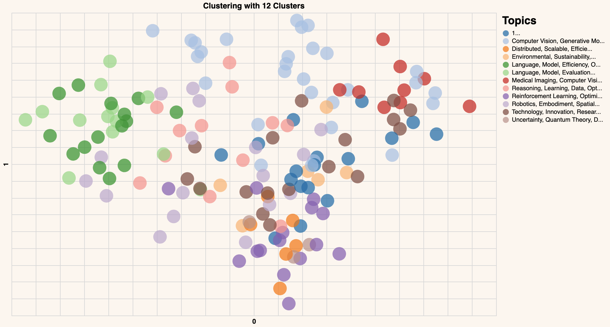
Congratulations! You have created the word embeddings and visualized them using a scatter plot, showing the overall structure of these papers.

Similarity Search Across Papers

Next, we’ll expand on the functionality we’ve built so far to make it possible to find papers related to a user-provided query.

As before, we’ll begin by defining our get_similarity function. It takes a target query and compares it to candidates to return the most relevant papers.

PYTHON
1from sklearn.metrics.pairwise import cosine_similarity
2
3def get_similarity(target,candidates):
4 # Turn list into array
5 candidates = np.array(candidates)
6 target = np.expand_dims(np.array(target),axis=0)
7
8 # Calculate cosine similarity
9 sim = cosine_similarity(target,candidates)
10 sim = np.squeeze(sim).tolist()
11 sort_index = np.argsort(sim)[::-1]
12 sort_score = [sim[i] for i in sort_index]
13 similarity_scores = zip(sort_index,sort_score)
14
15 # Return similarity scores
16 return similarity_scores

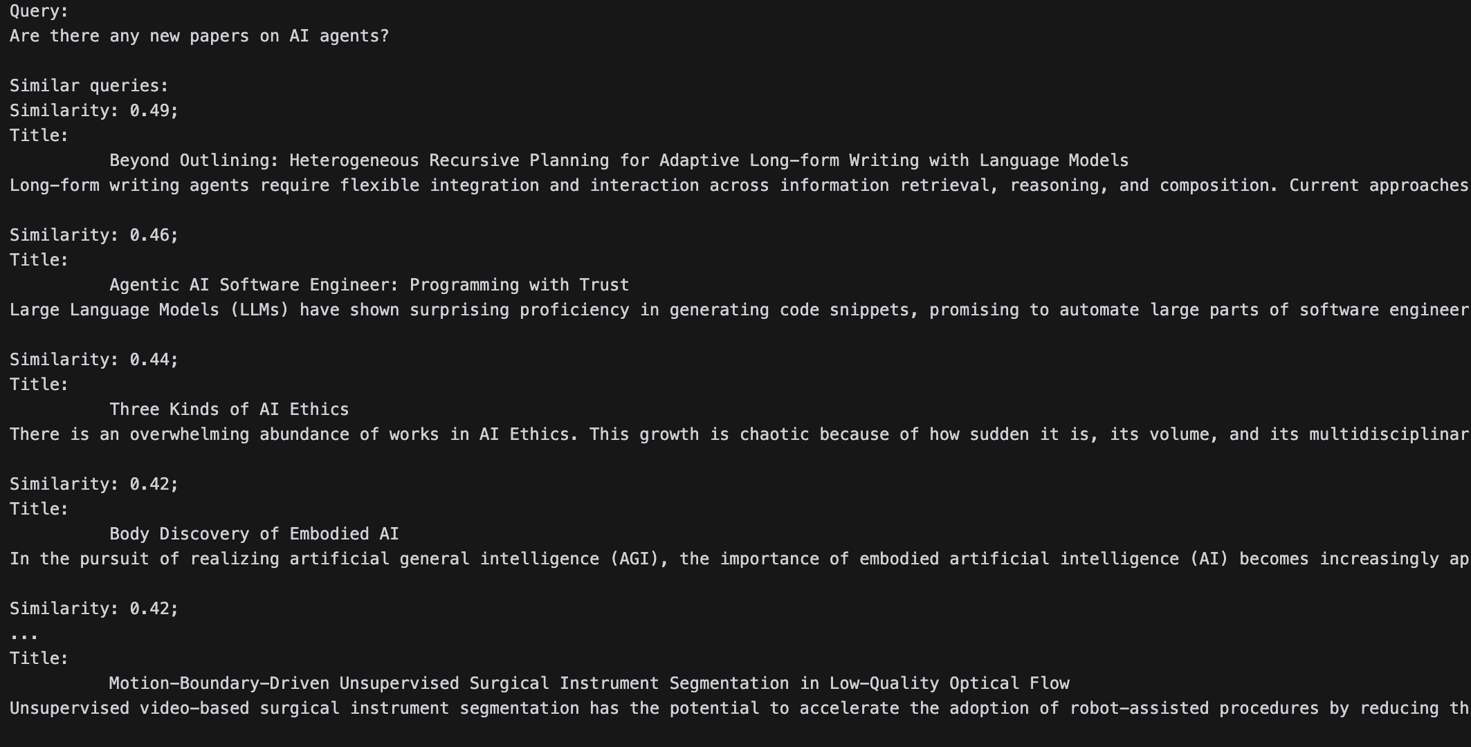
All we need now is to feed it a query and print out the top papers:

PYTHON
1# Add new query
2new_query = "Anything on AI personalities?"
3
4# Get embeddings of the new query
5new_query_embeds = get_embeddings(new_query)
6
7embeds = np.array(df_clust['text_embeds'].tolist()) # We defined these embeddings earlier and are pulling them out now for the function.
8
9# Get the similarity between the search query and existing queries
10similarity = get_similarity(new_query_embeds, embeds)
11#print(list(similarity))
12# View the top 5 articles
13print('Query:')
14print(new_query,'\n')
15
16print('Similar queries:')
17for idx,sim in similarity:
18 print(f'Similarity: {sim:.2f};')
19 print(df.iloc[idx]['titles'])
20 print(df.iloc[idx]['texts'])
21 print()

You should see something like this:

Similar papers

Conclusion

Let’s recap the NLP tasks implemented in this tutorial. You’ve created word embeddings, clustered those, and visualized them, then performed a semantic search to find similar papers. Cohere’s platform provides NLP tools that are easy and intuitive to integrate. You can create digital experiences that support powerful NLP capabilities like text clustering. It’s easy to register a Cohere account and get to an API key.

Built with